Plot the Inequality Curve

Plots the inequality curve $R(p) = Q(p/2) / Q(1 - p/2)$ over $p \in [0, 1]$, from either sampling survey data or a parametric distribution. The shaded area between the curve and the line $R(p) = 1$ equals the QRI.

Usage

plot_inequality_curve(
  y = NULL,
  qfunction = NULL,
  qfun_args = list(),
  weights = NULL,
  M = 200,
  type = 6,
  na.rm = TRUE,
  shade = TRUE,
  add = FALSE,
  col = "steelblue",
  shade_col = NULL,
  lwd = 1.5,
  lty = 1,
  legend_qri = TRUE,
  label = NULL,
  xlab = "p",
  ylab = "R(p)",
  main = "Inequality curve"
)

Arguments

y: Numeric vector of strictly positive values (e.g. income). Provide either y (empirical mode) or qfunction (parametric mode), not both.
qfunction: A parametric quantile function, e.g. qlnorm, qweibull. Provide either qfunction or y, not both.
qfun_args: Named list of additional arguments passed to qfunction (e.g. if qfunction == qlnorm, then provide list(meanlog = 9, sdlog = 0.6)).
weights: Numeric vector of sampling weights. Only used in estimation mode. If NULL, all observations are equally weighted.
M: Integer; number of grid points for evaluating $R(p)$ (default: 200).
type: Quantile estimation type (integer 4–9 or "HD"). Only used in empirical mode. Default: 6.
na.rm: Logical; remove missing values? Default: TRUE.
shade: Logical; if TRUE (default), shades the area between $R(p)$ and the equality line $R(p) = 1$. The shaded area equals the QRI.
add: Logical; if TRUE, adds the curve to an existing plot without redrawing axes. Each successive call appends a new entry to the legend on the right of the plot.
col: Colour of the inequality curve (default: "steelblue").
shade_col: Colour for the shaded area. Defaults to a transparent version of col.
lwd: Line width (default: 1.5).
lty: Line type (default: 1).
legend_qri: Logical; if TRUE (default), maintains a legend outside the plot area on the right, showing the QRI for each curve. When add = TRUE the new curve is appended below the previous entries.
label: Character string; overrides the auto-generated legend label ("QRI = X.XXXX"). Useful for giving curves descriptive names. Default: NULL (auto-label).
xlab: x-axis label (default: "p").
ylab: y-axis label (default: "R(p)").
main: Plot title (default: "Inequality curve").

Value

Beyond the plot, a named list with three elements:

p: Numeric vector of grid points in $[0, 1]$.
Rp: Numeric vector of $R(p)$ values at each grid point.
qri: The estimated QRI (area between the equality line and the curve).

The list is returned invisibly, meaning it is not printed to the console when the function is called without assignment. Assign the output to a variable (e.g. out <- plot_inequality_curve(...)) to inspect it.

Details

The inequality curve $R(p)$ plots the ratio of symmetric quantiles around the median: $$R(p) = \frac{Q(p/2)}{Q(1 - p/2)}, \quad p \in [0, 1]$$, against $p$. For a perfectly equal distribution $R(p) = 1$ for all $p$, and the curve coincides with the horizontal line at 1. The further the curve lies below the equality line, the more unequal the distribution. The QRI is the area between the equality line and the curve.

Boundary values $R(0) = 0$ and $R(1) = 1$ are set by convention (see Prendergast and Staudte (2018) ).

Multiple curves can be overlaid by calling the function repeatedly with add = TRUE. The legend outside the plot accumulates an entry for each curve automatically.

References

Prendergast LA, Staudte RG (2018). “A simple and effective inequality measure.” The American Statistician, 72, 328–343.

Scarpa S, Ferrante MR, Sperlich S (2025). “Inference for the quantile ratio inequality index in the context of survey data.” Journal of Survey Statistics and Methodology. doi:10.1093/jssam/smaf024 .

Examples

# -----------------------------------------------------------------
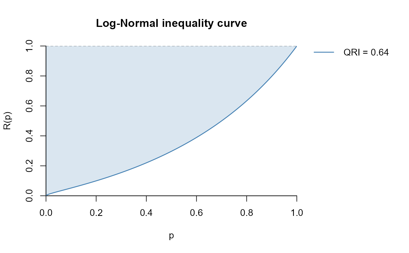
# Parametric mode: single curve
# -----------------------------------------------------------------
plot_inequality_curve(
  qfunction = qlnorm,
  qfun_args = list(meanlog = 9, sdlog = 0.9),
  main = "Log-Normal inequality curve"
)


# -----------------------------------------------------------------
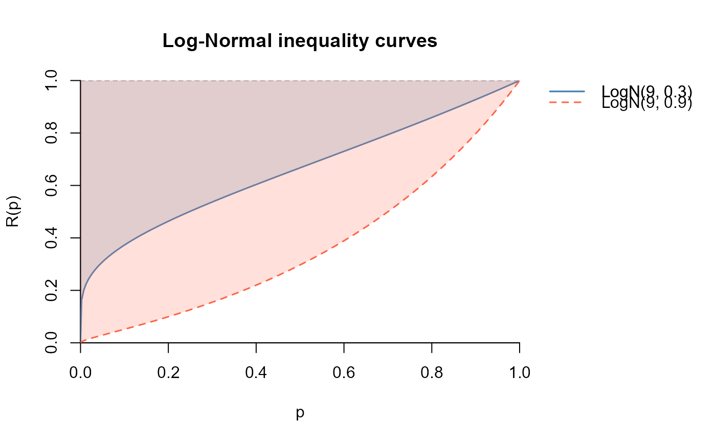
# Overlay multiple curves — legend accumulates automatically
# -----------------------------------------------------------------
plot_inequality_curve(
  qfunction = qlnorm,
  qfun_args = list(meanlog = 9, sdlog = 0.3),
  main  = "Log-Normal inequality curves",
  col   = "steelblue",
  label = "LogN(9, 0.3)"
)
plot_inequality_curve(
  qfunction = qlnorm,
  qfun_args = list(meanlog = 9, sdlog = 0.9),
  col   = "tomato", lty = 2, add = TRUE,
  label = "LogN(9, 0.9)"
)


# -----------------------------------------------------------------
# Empirical mode: survey data with sampling weights
# -----------------------------------------------------------------
data(synthouse)
out <- plot_inequality_curve(
  y       = synthouse$eq_income,
  weights = synthouse$weight,
  main    = "Inequality curve — synthouse"
)


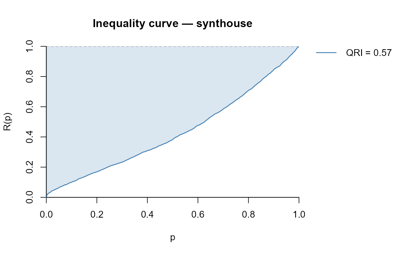# Inspect the returned list
out$qri          # estimated QRI
#> [1] 0.57
head(out$p)      # grid points
#> [1] 0.0000 0.0025 0.0075 0.0125 0.0175 0.0225
head(out$Rp)     # R(p) values
#>                0.125%     0.375%     0.625%     0.875%     1.125% 
#> 0.00000000 0.01523521 0.02547892 0.03099074 0.03567123 0.04309195