Introduction to inequantiles: Quantile-Based Inequality Measures for Survey Data

Overview

The inequantiles package provides tools for estimating quantiles and quantile-based economic inequality indicators from survey data, with full support for complex sampling designs.

The package offers comprehensive methods for:

Quantile ratio index (QRI): Estimation on superpopulations, complex survey data,and grouped data
Traditional quantile-based indicators: Quintile share ratio (QSR), Palma ratio, and percentile ratios (e.g., P90/P10), with flexible quantile estimator selection
Weighted quantile estimation: Estimation of quantiles choosing among multiple interpolation rules (types 4-9 plus HD) on complex sampling data
Linearization techniques: Estimation of influence function for QRI, QSR, Gini coefficient and quantiles
Grouped data support: Estimation of quantiles, QRI and Gini coefficient from frequency tables and grouped data when microdata are unavailable (e.g., fiscal data)
Sampling variance estimation for the cited indicators (and custom functions) via rescaled bootstrap method

All functions are demonstrated using synthetic survey data included in the package.

Installation

# Install from GitHub
devtools::install_github("silviascarpa/inequantiles")

library(inequantiles)

Import synthetic survey data

The dataset synthouse was synthetically generated to mimic typical survey dataset like Italian EU-SILC. It contains basic information at the individual and household level, including geographical information, sampling weights and equivalised disposable income.

data(synthouse)
head(synthouse)
#>    person_id    hh_id NUTS1 NUTS2   NUTS3 municipality age age_class gender
#> 1 HH000001P1 HH000001     N   N01  N01005   N010050010  39     35-49      1
#> 2 HH000001P2 HH000001     N   N01  N01005   N010050010  38     35-49      2
#> 3 HH000001P3 HH000001     N   N01  N01005   N010050010  15     15-17      1
#> 4 HH000001P4 HH000001     N   N01  N01005   N010050010  13      0-14      2
#> 5 HH000002P1 HH000002    NE  NE06 NE06004  NE060040007  37     35-49      2
#> 6 HH000003P1 HH000003     N   N05  N05003   N050030007  54     50-64      2
#>   education_level employment_status hh_size hh_type eq_income hh_income
#> 1             Low          Employed       4  Family  10430.70  23990.61
#> 2          Medium          Employed       4  Family  10430.70  23990.61
#> 3            <NA>           Student       4  Family  10430.70  23990.61
#> 4            <NA>           Student       4  Family  10430.70  23990.61
#> 5          Medium          Employed       1  Single  36588.27  36588.27
#> 6             Low          Employed       2  Couple  13390.50  20085.75
#>   oecd_scale     weight
#> 1        2.3   83.66134
#> 2        2.3   83.66134
#> 3        2.3   83.66134
#> 4        2.3   83.66134
#> 5        1.0  167.24423
#> 6        1.5 1419.28854

Theoretical Background

Unlike moment-based inequality indicators (e.g., the Gini coefficient), which are highly sensitive to large values in the long tails, indicators which are based solely on quantiles are remarkably resistant to anomalous observations and high distribution skewness.

The core of the inequantiles package is the quantile ratio index (QRI), an indicator that provides a robust measure of inequality, even in small samples, as it considers the entire distribution and is solely based on quantiles.

The Quantile Ratio Index (QRI)

The QRI was introduced by Prendergast and Staudte (2018) as a simple, effective inequality measure of economic inequality. The QRI

Considers the entire distribution
Depends solely on quantiles
Is robust to extreme values
Does not require a priori choice of specific percentiles
Is nonparametric

For a continuous non-negative random variable $Y$ with cumulative distribution function $F(y)$ and quantile function $Q(p) = F^{-1}(p)$, $0 \leq p \leq 1$, define the ratio between symmetric quantiles as:

\[R(p) = \frac{Q(p/2)}{Q(1-p/2)}, \quad \leq p \leq 1.\] $R(p)$ in a non-decreasing function between 0 and 1, which takes value 1 for any $0 \leq p \leq 1$ when income (or another economic variable with poisitive support) is equally distributed among the individuals.

The QRI is then defined as:

\[\text{QRI} = 1 - \int_0^1 R(p) \, dp = 1 - \int_0^1 \frac{Q(p/2)}{Q(1-p/2)} \, dp.\]

The QRI ranges from 0 (perfect equality) to 1 (maximum inequality). It measures the area between the equi-distribution line ($R(p) = 1$ for all $p$) and the actual inequality curve. This can be easily visualised by the following plots:

### Log-Normal distribution
plot_inequality_curve(qfunction = qlnorm, qfun_args = list(meanlog = 9, sdlog = 0.3),
                      col   = "tomato", lty = 2, label = "LogN(sigma=0.3)")
plot_inequality_curve(qfunction = qlnorm, qfun_args = list(meanlog = 9, sdlog = 1.9),
                      col   = "blue", lty = 2, add = TRUE, label = "LogN(sigma=1.9)")
plot_inequality_curve(qfunction = qlnorm, qfun_args = list(meanlog = 9, sdlog = 3.9),
                      col   = "green", lty = 2, add = TRUE, label = "LogN(sigma=3.9)")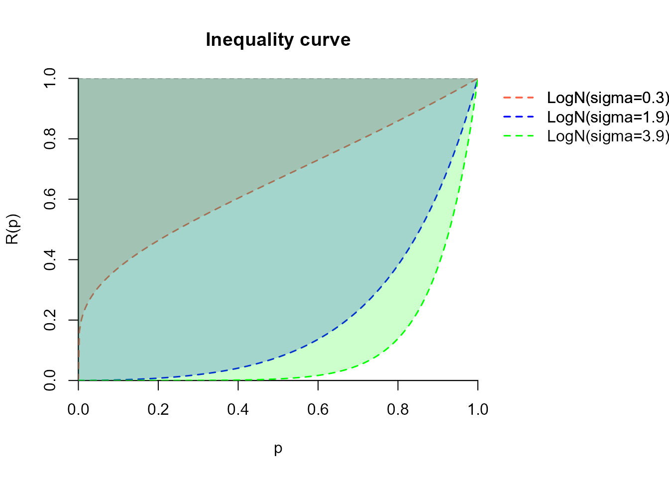

For superpopulation models defined by theoretical parametric distributions with known quantile functions, you can compute the exact QRI as:

# Log-normal distribution
superpop_qri(qfunction = qlnorm, meanlog = 9, sdlog = 0.2)
#> [1] 0.2534457
superpop_qri(qfunction = qlnorm, meanlog = 9, sdlog = 1.7)
#> [1] 0.7818321
superpop_qri(qfunction = qlnorm, meanlog = 9, sdlog = 3.2)
#> [1] 0.8781747

# Weibull distribution
superpop_qri(qfunction = qweibull, shape = 2, scale = 30000)
#> [1] 0.522862
superpop_qri(qfunction = qweibull, shape = 1.5, scale = 30000)
#> [1] 0.6003122

Consider now a finite population $U = \{1, \ldots, N\}$, from which a random sample $s$ of size $n$ is selected, typically collected with a complex sampling design $p(s) = Pr(S = s)$, $\forall s \subseteq U$. Let $y_j$, $j \in s$, be the observed values of the variable of interest, with $y_{(1)}, \ldots, y_{(n)}$ denoting its order statistics. Assume that the sample is drawn according to a certain sampling scheme, with inclusion probability $\pi_j = Pr(j \in s)$. The corresponding sampling weight $w_j$ is obtained by the inversion of the inclusion probability, plus, when required, some adjustments for non-response and calibration. Let $W_j = \sum_{i \in s} w_i \mathbf{1}(i \leq j)$ denote the cumulative sum of weights up to ordered observation $j$. Let $\widehat{Q}(p)$ be the $p$ quantile estimator; how to estimate the quantiles on complex sampling data will be treated in the following sections. For survey data from a finite population, Scarpa, Ferrante, and Sperlich (2025) estimate the QRI using a grid of $M$ points on $(0, 1)$ as

\[ \widehat{\text{QRI}} = \frac{1}{M} \sum_{m=1}^M \left(1 - \frac{\widehat{Q}(p_m/2)}{\widehat{Q}(1-p_m/2)}\right) \]

where $p_m = (m-0.5)/M$, for $ m = 1, , M$. By default, $M = 100$.

qri(y = synthouse$eq_income, weights = synthouse$weight, M = 100)
#> [1] 0.5690895

$\widehat{\text{QRI}}$ is strictly sensitive to the choice of the quantile estimator, especially in small samples.

Quantile estimators

The $p$ quantile estimator can be expressed as a weighted average of order statistics,

\[ \widehat{Q}(p)=y_{(k-1)}+ \left(y_{(k )} - y_{(k- 1)}\right) \left(\frac{p - \widehat{r}_{k - 1 }}{\widehat{r}_{k} - \widehat{r}_{k - 1}} \right), \label{eq:quantiles complessi} \]

where $\widehat{r}_{k}$ indicates the estimator of the cdf, namely the plotting position, and the selected order $k$ is such that $W_{k-1} - m_{k-1} < W_n p < W_{k} - m_k$, where $m_k$ is determined by the interpolation method between adjacent data points. Linear interpolation between the points $(\widehat r, y_{(k)})$ gives a quantile estimator for complex sampling data. For $p=0$ and $p=1$, define $\widehat{Q} (0)=y_{(1)}$ and $\widehat{Q}(1)=y_{(n)}$.

The csquantile() function extends standard quantile estimation through the R function quantile() to survey data. It adapts the methods described in Hyndman and Fan (1996) to weighted data. The possible interpolation rules are summarised in the table below (see Scarpa, Ferrante, and Sperlich (2025) for further details):

**Table 1:** Quantile estimators incorporating sampling weights.
Estimator	$\widehat{r}_k$	$\widehat{m}_k$	$k$
$\widehat{Q}_4(p)$	$\frac{W_k}{W_n}$	0	$W_{k-1} \le W_n p \lt W_k$
$\widehat{Q}_5(p)$	$\frac{W_k-\frac{1}{2}w_k}{W_n}$	$\frac{w_k}{2}$	$W_{k-1} - \frac{w_{k-1}}{2} \le W_n p \lt W_{k} - \frac{w_{k}}{2}$
$\widehat{Q}_6(p)$	$\frac{W_k}{W_n+w_n}$	$w_np$	$W_{k-1} \le (W_n + w_n)p \lt W_{k}$
$\widehat{Q}_7(p)$	$\frac{W_{k-1}}{W_{n-1}}$	$w_k - w_np$	$W_{k-2} \le W_{n-1}p \lt W_{k-1}$
$\widehat{Q}_8(p)$	$\frac{W_k-\frac{1}{3}w_k}{W_n+rac{w_n}{3}}$	$\frac{w_k}{3} + \frac{w_n}{3}p$	$W_{k-1} - \frac{w_{k-1}}{3} \le (W_{n} - \frac{w_n}{3})p \lt W_{k} - \frac{w_k}{3}$
$\widehat{Q}_9(p)$	$\frac{W_k-\frac{3}{8}w_k}{W_n+rac{1}{4}w_n}$	$\frac{3}{8}w_k + \frac{w_n}{4}p$	$W_{k-1} - \frac{3w_{k-1}}{8} \le (W_{n} + \frac{w_{n}}{4})p \lt W_{k} - \frac{3w_{k}}{8}$

They can be easily compued on survey data, as:

# Compute weighted quartiles
csquantile(y = synthouse$eq_income,
           weights = synthouse$weight,
           probs = c(0.25, 0.5, 0.75),
           type = 4)
#>      25%      50%      75% 
#> 12353.29 20014.13 32222.45
csquantile(y = synthouse$eq_income,
           weights = synthouse$weight,
           probs = c(0.25, 0.5, 0.75),
           type = 7)
#>      25%      50%      75% 
#> 12353.29 20019.77 32224.95

# Compare without considering the sampling weights
csquantile(synthouse$eq_income, probs = c(0.25, 0.5, 0.75), type = 4)
#>      25%      50%      75% 
#> 12910.30 20428.45 32528.88

An extension of the Harrell-Davis estimator to survey data is also provided, as $\widehat{Q}_{HD}(p)=\sum_{j \in s} \widehat{\mathcal{W}}_{j}(p) y_{(j)}$, where

\[ \begin{aligned} \widehat{\mathcal{W}}_{j}(p) = & \, b_{(W_{j} / W_n)}\{(W_n+ w_n) p, W_n - (W_n+ w_n)p + w_n\} \\ & - b_{(W_{j - 1}/ W_n)}\{(W_n+ w_n) p, W_n - (W_n+ w_n)p + w_n\} \end{aligned} \]

# Harrell-Davis weighted median
csquantile(y = synthouse$eq_income,
           weights = synthouse$weight,
           probs = 0.5,
           type = "HD")
#>      50% 
#> 20017.37

Differences among the quantle estimators are particularly evident in small samples and in the distribution tails, as demonstrated in the following example:

# Compare different quantile types by NUTS3
types <- c(4, 5, 6, 7, 8, 9, "HD")
areas <- unique(synthouse$NUTS3)

# Function to compute QRI for all types in one area
compare_quantiles <- function(region_code, data = synthouse) {
  idx <- which(data$NUTS3 == region_code)
  
  results <- sapply(types, function(t) {
    csquantile(y = data$eq_income[idx], 
        weights = data$weight[idx], 
        type = t,
        probs = 0.95)
  })
  
  return(results)
}

# Compute for all areas
results_quantiles <- sapply(areas, compare_quantiles)
rownames(results_quantiles) <- types
colnames(results_quantiles) <- areas


## === Quantile estimators for Each NUTS3 Region ==="
print(head(t(results_quantiles), n = 10))
#>                4        5        6        7        8        9       HD
#> N01005  70988.83 75538.32 87604.07 69761.89 80343.39 79093.40 76388.02
#> NE06004 50988.47 50988.47 50988.47 50992.05 50988.47 50988.47 50988.47
#> N05003  81116.08 82948.72 81211.01 83560.96 82496.53 82633.53 81370.54
#> NE06002 47742.34 47749.81 47749.81 47749.81 47749.81 47749.81 47749.81
#> N02004  52599.79 53137.63 52644.75 53559.00 52883.63 52956.29 52818.39
#> NO02004 66674.78 66674.78 67773.72 61032.04 66904.21 66771.79 66674.78
#> NO03002 67724.83 71393.13 71459.35 71351.81 71411.51 71406.64 72491.41
#> N06004  45313.69 45317.87 45313.69 45706.20 45313.69 45313.69 45313.69
#> NE02004 57268.49 57299.09 57303.00 57297.80 57299.86 57299.64 57279.50
#> S04005  58411.94 62602.84 60288.65 62670.74 61561.74 61786.33 62670.69

The package supports multiple quantile estimation methods (types 4-9 and Harrell-Davis) into quantile-based inequality indicators estimators. Rule type = 6is recommended for the QRI, as it is been shown by Scarpa, Ferrante, and Sperlich (2025) to lead to the least biased estimates.

# Compute weighted QRI
qri(y = synthouse$eq_income, 
    weights = synthouse$weight, 
    type = 6)  # Type 6 quantile estimator (default)
#> [1] 0.5690895

QRI estimator sampling variance

For complex surveys, the rescaled bootstrap method (Rao and Wu 1988; Rao, Wu, and Yue 1992) is recommended for the estimation of the QRI estimator sampling variance, as demonstrated by Scarpa, Ferrante, and Sperlich (2025). This can be easily estimated on data collected through two-stage stratified sampling design as

# Pseudo-code for rescaled bootstrap for the estimation of the sampling variance of the QRI estimator
var_qri <- rescaled_bootstrap(
  data = synthouse,
  y = "eq_income",
  strata = "NUTS2",
  psu = "municipality",
  weights = "weight",
  estimator = qri,
  by_strata = TRUE,
  B = 100,
  seed = 456)

Other Inequality Indicators

Most common quantile-based inequality indicators in the literature are the quintile share ratio (QSR), the Palma ratio and the interdecile ratios. All estimators implemented in this package allow the user to choose the quantile estimation method via the type argument.

The QSR compares the income share of the top 20% to the bottom 20%. Its estimator is defined as

\[ \widehat{{QSR}} = \frac{\sum_{j \in s}w_j y_j \mathbf{1}\left\{ y_j \geq \widehat{Q}(0.8)\right\} }{\sum_{j \in s} w_j y_j\mathbf{1}\left\{ y_j \leq \widehat{Q}(0.2)\right\} } \ . \]

# Compute QSR
qsr(y = synthouse$eq_income, 
    weights = synthouse$weight, type = 4)
#> [1] 7.023932

Palma Ratio

The Palma ratio compares the top 10% to the bottom 40% aggregated income: \[ \widehat{{Palma}} = \frac{\sum_{j \in s}w_j y_j \mathbf{1}\left\{ y_j \geq \widehat{Q}(0.9)\right\} }{\sum_{j \in s} w_j y_j\mathbf{1}\left\{ y_j \leq \widehat{Q}(0.4)\right\} } \ . \]

# Compute Palma ratio
palma_ratio(y = synthouse$eq_income, 
            weights = synthouse$weight, type = 7)
#> [1] 1.578482

Percentile Ratios

Very often National Statistical Offices measure inequality using ratios between percentiles, for example: \[ \widehat{{P}90/{P}10} = \frac{\widehat{Q}(p=0.9)}{\widehat{Q}(p=0.1)} \]

Default the P90/P10 is estimated.

# P90/P10 ratio
ratio_quantiles(y = synthouse$eq_income,
                weights = synthouse$weight,
                type = 7)
#>  P90/P10 
#> 5.918233

# P75/P25 ratio
ratio_quantiles(y = synthouse$eq_income,
                weights = synthouse$weight,
                prob_numerator = 0.75,
                prob_denominator = 0.25, type = 6)
#> P75/P25 
#> 2.60845

Comparing Indicators Across Groups

Multiple inequality indicators exist in the literature, each capturing different aspects of the economic distribution. Different indicators may provide complementary perspectives on inequality, so researchers should choose the most appropriate measure based on their specific research questions and the distributional features of interest.

The inequantiles() function computes all quantile-based indicators at once, or any subset of them, among QRI, QSR, Palma ratio and interquantiles ratio.

# Compare all indicators
inequantiles(y          = synthouse$eq_income,
             weights    = synthouse$weight,
             indicators = "all")
#> Quantile-based inequality indicators
#> -------------------------------------
#>        Estimate
#> qri      0.5691
#> qsr      7.0161
#> palma    1.5787
#> p90p10   5.9206

Standard errors can be obtained via the rescaled bootstrap by setting se = TRUE. Note that this requires specifying the survey design variables (strata, and optionally psu and N_h).

# QRI and QSR with their standard errors for one region via rescaled bootstrap
nord <- synthouse[synthouse$NUTS1 == "N", ]

qri_qsr <- inequantiles(
  y       = nord$eq_income,
  weights = nord$weight,
  indicators = c("qri", "qsr"),
  se      = TRUE,
  data    = nord,
  strata  = "NUTS2",
  psu     = "municipality",
  B       = 200,
  seed    = 42
)

Linearization techniques via influence function

The package provides linearization methods using the influence function estimation for some measures.

The quantile estimator influence function (IF) is measured in Osier (2009) as \[ {I}(\widehat{Q}(p))_{k} = \frac{p - \mathbb{1}(y_k \leq \widehat{Q}(p)) }{\widehat{F}'(\widehat{Q}(p)) N}, \] where $\widehat{F}'(y) = \frac{1}{\widehat N}\frac{1}{h \sqrt{2 \pi}} \sum_{j \in s} w_j \operatorname{exp} \left\{-\frac{(y - y_j)^2}{2h^2} \right\}$.

The QSR estimator IF, as demonstrated by Langel and Tillé (2011), can be computed as \[ \begin{split} I(\widehat{QSR})_{k} &= \frac{y_k-\left\{0.8 \widehat{Q}(0.8)-\left(\widehat{Q}(0.8)-y_k\right) \mathbf{1}\left[y_k \leq \widehat{Q}(0.8)\right]\right\}}{\widehat{Y}_{0.2}} \\ &\quad - \frac{\left(\widehat{Y}-\widehat{Y}_{0.8}\right)\left\{0.2 \widehat{Q}(0.2)-\left(\widehat{Q}(0.2)-y_k\right) \mathbf{1}\left[y_k \leq \widehat{Q}(0.2)\right]\right\}}{\widehat{Y}_{0.2}^2} \end{split} \]

where $\hat{Y}_{\alpha} = \sum_{j \in s} w_j y_j \mathbf{1}[y_k \leq \widehat{Q}(\alpha)]$.

Scarpa, Ferrante, and Sperlich (2025) demonstrated that the QRI IF can be estimated as \[ \begin{split} {I}(\widehat{QRI})_{k} &= - \int_0^1 \frac{\left(\frac{\frac{p}{2} - \mathbb{1}(y_k \leq \widehat{Q}(p/2))}{\widehat{F}'(\widehat{Q}(p/2)) \widehat N}\right) \widehat{Q}(1-p/2) - \left(\frac{(1 - \frac{p}{2}) - \mathbb{1}(y_k \leq \widehat{Q}(1-p/2))}{\widehat{F}'(\widehat{Q}(1-p/2)) \widehat N}\right) \widehat{Q}(p/2)}{ \widehat{Q}(1-p/2)^2}dp \ . \end{split} \]

The Gini coefficient IF can be approximated as (see Langel and Tillé (2013)) as \[ {I}(\widehat{G})_{k} =\frac{1}{\hat{N} \hat{Y}}\left\{2 W_k\left(y_k-\hat{\bar{Y}}_k\right)+\hat{Y}-\hat{N} y_k-\hat{G}\left(\hat{Y}+y_k \hat{N}\right)\right\} \] \[ \text{with} \qquad \hat{Y} = \sum_{j \in s}w_j y_j; \quad \hat{\bar{Y}}_j=\frac{\sum_{l \in S} w_l y_l 1\left(W_l \leqslant W_j\right)}{W_k}. \]

Comparison of the influence function values

# Select a subset for clearer visualization
n_obs <- 200
set.seed(123)
idx <- sample(nrow(synthouse), n_obs)

# Extract data
y_subset <- synthouse$eq_income[idx]
w_subset <- synthouse$weight[idx]

# Order income values (for ease of representation, see the plots later)
order_idx <- order(y_subset)
y_ordered <- y_subset[order_idx]      # Order the data
w_ordered <- w_subset[order_idx]      

# Compute the IF for some indicators
if_gini_vals <- if_gini(y_ordered, w_ordered)
if_qri_vals <- if_qri(y_ordered, w_ordered, type = 6)
if_qsr_vals <- if_qsr(y_ordered, w_ordered, type = 4)
if_q50_vals <- if_quantile(y_ordered, w_ordered, probs = 0.5, type = 6)

# Create the plot
library(ggplot2)
#> Warning: package 'ggplot2' was built under R version 4.4.3
library(scales)
#> Warning: package 'scales' was built under R version 4.4.3

# 
plot_df <- data.frame(
  Income = rep(y_ordered, 4),
  IF_Value = c(
    if_qri_vals,   # ← Già ordinato
    if_qsr_vals,   # ← Già ordinato
    if_gini_vals,  # ← Già ordinato
    if_q50_vals    # ← Già ordinato
  ),
  Indicator = rep(c("QRI", "QSR", "Gini", "Median"), each = n_obs)
)

ggplot(plot_df, aes(x = Income, y = IF_Value, color = Indicator)) +
  geom_line(linewidth = 0.8, alpha = 0.7) +
  geom_hline(yintercept = 0, linetype = "dashed", color = "gray40") +
  facet_wrap(~ Indicator, scales = "free_y", ncol = 2) +
  scale_x_continuous(labels = scales::comma) +
  labs(
    title = "Influence Functions: How Each Observation Affects the Estimate",
    subtitle = paste("Based on", n_obs, "randomly sampled households"),
    x = "Equivalized Income",
    y = "Influence Function Value",
  ) +
  theme_minimal(base_size = 11) +
  theme(
    legend.position = "none",
    strip.text = element_text(face = "bold", size = 11),
    plot.title = element_text(face = "bold", size = 13),
    plot.subtitle = element_text(color = "gray40"),
    panel.grid.minor = element_blank()
  )

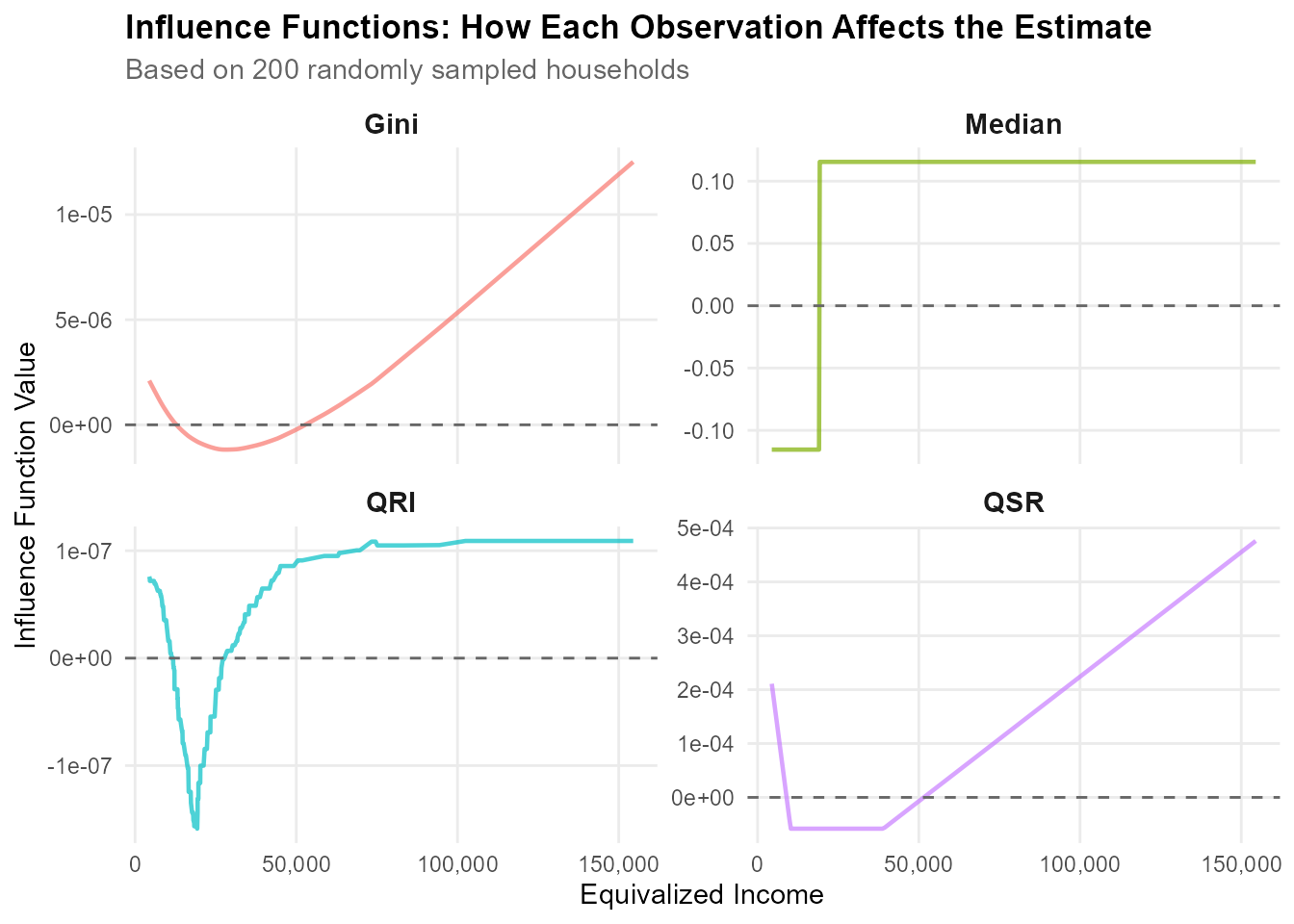
We observe that

Gini Coefficient:

Shows generally increasing unbounded pattern with income
Less sensitive to low incomes

QRI:

Balanced influence across the entire distribution
Jump around the median
Upper bound as income increases
More robust than the other inequality indicators

Median:

Step function that admits only two values
Robust but ignores most of the distribution

QSR:

Sharp discontinuities at $Q(0.2)$ and $Q(0.8)$
Near-zero influence in the middle 60% of distribution
High sensitivity to observations at boundary quantiles

Grouped Data Functions

When only frequency tables are available (common with administrative or tax data), the package provides specialized functions.

Consider grouped data divided into $L$ classes with known boundaries, observed frequencies $f_1, \ldots, f_L$ and total amounts $Y_1, \ldots, Y_L$. Let:

$L_l$ be the lower bound of the $l$-th class
$U_l$ be the upper bound of the $l$-th class
$h_l = U_l - L_l$ be the $l$-th class width
$N = \sum_{i=1}^{L} f_i$ be the total frequency
$C_{l} = \sum_{i=1}^{l} f_i$ be the cumulative frequency up to the $l$-th class
$c_l = Y_l / \sum_{i=1}^{L} Y_i$ is the share in group $l$
$s_l = \sum_{k=1}^{l} c_k$ is the cumulative share up to group $l$
$p_l = f_l / \sum_{i=1}^{L} f_i$ be the population share of group $l$
$u_l = \sum_{k=1}^{l} p_k$ is the cumulative population share up to group $l$
$s_0 = u_0 = 0$ by convention

For example

# Example: Income distribution in frequency table format
income_freq <- c(120, 180, 150, 80, 40, 20, 10)
income_tot <- c(18800, 16300, 44700, 33900, 21500, 22100, 98300)
income_lower <- c(0, 15000, 30000, 45000, 60000, 80000, 100000)
income_upper <- c(15000, 30000, 45000, 60000, 80000, 100000, 150000)

Quantile Computation for Grouped Data

The quantile class for the ${p}$-th quantile is the first class ${l}$ such that:

\[ {l = min\{l: C_l \geq pN \}} \]

The ${p}$-th quantile ${Q(p)}$ is then estimated by linear interpolation within the quantile class:

\[ {\widetilde{Q}(p) = L_l + \frac{(pN - C_{l-1})}{f_l} \cdot h_l} \]

# Estimate quantiles from grouped data
quantile_grouped(freq = income_freq,
                 lower_bounds = income_lower,
                 upper_bounds = income_upper,
                 probs = c(0.25, 0.5, 0.75))
#>  25 %  50 %  75 % 
#> 17500 30000 45000

QRI for Grouped Data

By using the quantile measure for grouped data, the QRI is approximated as:

\[ {{QRI}} \approx \frac{1}{M}\sum_{m=1}^{M}\left(1 - \frac{\widetilde{Q}(p_m/2)}{\widetilde{Q}(1 - p_m/2)}\right) \]

# Compute QRI from grouped data
qri_grouped(freq = income_freq, 
            lower_bounds = income_lower, 
            upper_bounds = income_upper,
            M = 100)
#> [1] 0.5888192

Gini coefficient from Grouped Data

The Gini coefficient is approximated by linear interpolation of cumulative shares, as:

\[ {G \approx 1 - \sum_{l=1}^{L} (s_l + s_{l-1})(u_l - u_{l-1})} \]

# Estimate quantiles from grouped data
gini_grouped(Y = income_tot, freq = income_freq)
#> [1] 0.5787167

Getting Help

If you encounter issues or have questions:

Open an issue on GitHub
Check the function documentation: ?qri, ?csquantile, etc.
Contact the maintainer: silvia.scarpa@unimore.it

References

Session Info

sessionInfo()
#> R version 4.4.1 (2024-06-14 ucrt)
#> Platform: x86_64-w64-mingw32/x64
#> Running under: Windows 11 x64 (build 26200)
#> 
#> Matrix products: default
#> 
#> 
#> locale:
#> [1] LC_COLLATE=Italian_Italy.utf8  LC_CTYPE=Italian_Italy.utf8   
#> [3] LC_MONETARY=Italian_Italy.utf8 LC_NUMERIC=C                  
#> [5] LC_TIME=Italian_Italy.utf8    
#> 
#> time zone: Europe/Rome
#> tzcode source: internal
#> 
#> attached base packages:
#> [1] stats     graphics  grDevices utils     datasets  methods   base     
#> 
#> other attached packages:
#> [1] scales_1.4.0            ggplot2_4.0.2           kableExtra_1.4.0       
#> [4] knitr_1.51              inequantiles_0.0.0.9000
#> 
#> loaded via a namespace (and not attached):
#>  [1] gtable_0.3.6       jsonlite_2.0.0     dplyr_1.1.4        compiler_4.4.1    
#>  [5] tidyselect_1.2.1   xml2_1.5.2         stringr_1.6.0      jquerylib_0.1.4   
#>  [9] systemfonts_1.3.1  textshaping_1.0.0  yaml_2.3.12        fastmap_1.2.0     
#> [13] R6_2.6.1           labeling_0.4.3     generics_0.1.4     rbibutils_2.4.1   
#> [17] htmlwidgets_1.6.4  tibble_3.2.1       desc_1.4.3         svglite_2.2.2     
#> [21] pillar_1.10.1      bslib_0.10.0       RColorBrewer_1.1-3 rlang_1.1.7       
#> [25] cachem_1.1.0       stringi_1.8.7      xfun_0.56          S7_0.2.1          
#> [29] fs_1.6.7           sass_0.4.10        viridisLite_0.4.2  cli_3.6.5         
#> [33] withr_3.0.2        pkgdown_2.1.3      magrittr_2.0.4     Rdpack_2.6.6      
#> [37] digest_0.6.39      grid_4.4.1         rstudioapi_0.18.0  lifecycle_1.0.5   
#> [41] vctrs_0.7.1        evaluate_1.0.5     glue_1.8.0         farver_2.1.2      
#> [45] ragg_1.5.0         rmarkdown_2.30     pkgconfig_2.0.3    tools_4.4.1       
#> [49] htmltools_0.5.9

Hyndman, Rob J., and Yanan Fan. 1996. “Sample Quantiles in Statistical Packages.” The American Statistician 50: 361–65.

Langel, Matti, and Yves Tillé. 2011. “Statistical Inference for the Quintile Share Ratio.” Journal of Statistical Planning and Inference 141: 2976–85.

———. 2013. “Variance Estimation of the Gini Index: Revisiting a Result Several Times Published.” Journal of the Royal Statistical Society Series A 176: 521–40.

Osier, Guillaume. 2009. “Variance Estimation for Complex Indicators of Poverty and Inequality Using Linearization Techniques.” Survey Research Methods 3: 167–95.

Prendergast, Luke A., and Robert G. Staudte. 2018. “A Simple and Effective Inequality Measure.” The American Statistician 72: 328–43.

Rao, John N.K., and Chien F.J. Wu. 1988. “Resampling Inference with Complex Survey Data.” Journal of the American Statistical Association 83: 231–41.

Rao, John N.K., Chien F.J. Wu, and Kim Yue. 1992. “Some Recent Work on Resampling Methods for Complex Surveys.” Survey Methodology 18: 209–17.

Scarpa, Silvia, Maria Rosaria Ferrante, and Stefan Sperlich. 2025. “Inference for the Quantile Ratio Inequality Index in the Context of Survey Data.” Journal of Survey Statistics and Methodology. https://doi.org/10.1093/jssam/smaf024.

Estimator	\(\widehat{r}_k\)	\(\widehat{m}_k\)	\(k\)
\(\widehat{Q}_4(p)\)	\(\frac{W_k}{W_n}\)	0	\(W_{k-1} \le W_n p \lt W_k\)
\(\widehat{Q}_5(p)\)	\(\frac{W_k-\frac{1}{2}w_k}{W_n}\)	\(\frac{w_k}{2}\)	\(W_{k-1} - \frac{w_{k-1}}{2} \le W_n p \lt W_{k} - \frac{w_{k}}{2}\)
\(\widehat{Q}_6(p)\)	\(\frac{W_k}{W_n+w_n}\)	\(w_np\)	\(W_{k-1} \le (W_n + w_n)p \lt W_{k}\)
\(\widehat{Q}_7(p)\)	\(\frac{W_{k-1}}{W_{n-1}}\)	\(w_k - w_np\)	\(W_{k-2} \le W_{n-1}p \lt W_{k-1}\)
\(\widehat{Q}_8(p)\)	\(\frac{W_k-\frac{1}{3}w_k}{W_n+rac{w_n}{3}}\)	\(\frac{w_k}{3} + \frac{w_n}{3}p\)	\(W_{k-1} - \frac{w_{k-1}}{3} \le (W_{n} - \frac{w_n}{3})p \lt W_{k} - \frac{w_k}{3}\)
\(\widehat{Q}_9(p)\)	\(\frac{W_k-\frac{3}{8}w_k}{W_n+rac{1}{4}w_n}\)	\(\frac{3}{8}w_k + \frac{w_n}{4}p\)	\(W_{k-1} - \frac{3w_{k-1}}{8} \le (W_{n} + \frac{w_{n}}{4})p \lt W_{k} - \frac{3w_{k}}{8}\)

Silvia Scarpa

2026-04-14

Overview

Installation

Import synthetic survey data

Theoretical Background

The Quantile Ratio Index (QRI)

Quantile estimators

QRI estimator sampling variance

Other Inequality Indicators

Palma Ratio

Percentile Ratios

Comparing Indicators Across Groups

Linearization techniques via influence function

Comparison of the influence function values

Grouped Data Functions

Quantile Computation for Grouped Data

QRI for Grouped Data

Gini coefficient from Grouped Data

Getting Help

References

Session Info

Introduction to inequantiles: Quantile-Based Inequality Measures for Survey Data

Silvia Scarpa

2026-04-14

Overview

Installation

Import synthetic survey data

Theoretical Background

The Quantile Ratio Index (QRI)

Quantile estimators

QRI estimator sampling variance

Other Inequality Indicators

Quintile Share Ratio (QSR)

Palma Ratio

Percentile Ratios

Comparing Indicators Across Groups

Linearization techniques via influence function

Comparison of the influence function values

Grouped Data Functions

Quantile Computation for Grouped Data

QRI for Grouped Data

Gini coefficient from Grouped Data

Getting Help

References

Session Info